Flow Input Options#
HydroGenerate allows entering flow in multiple formats. More advance functionality is avaliable when a time series of flow is avaliable.
Using hydropower_type = Diversion allows computing hydropower potential for a diversion or run-of-river project.
from HydroGenerate.hydropower_potential import calculate_hp_potential
import numpy as np
import pandas as pd
import matplotlib.pyplot as plt
Flow as a numpy array#
When flow is a numpy array, HydroGenerate can select a design flow and calculate nameplate capacity, effiiency, and head losses for the given vlues of flow.
The file data_test.csv used in the examples below is available in the ./examples/ directory of the repository. The Jupyter notebook files for all examples are located in the jugc-docs branch, within the docs folder.
# Head, power, and length of penstock are known. Multiple values of flow are available, the design flow is not known.
# In this scenario HydroGenerate will select a turbine, compute efficiency for the given flow values,
# design flow based on a percent of exceedance, penstock diameter (assuming steel if no material is given),
# head loss for all flows, rater power,
# power a given range of flow,

flow = pd.read_csv('data_test.csv')['discharge_cfs'].to_numpy() # cfs
head = 20 # ft
power = None
penstock_length = 50 # ft
hp_type = 'Diversion'
pctime_runfull= 20 # percent of time the turbine is running full - default is 30%

# Note: decreasing the percent of time the turbine will run full will result in a
# larger system (rated power and cost)

hp = calculate_hp_potential(flow= flow, rated_power= power, head= head,
                           penstock_headloss_calculation= True,
                           hydropower_type= hp_type, penstock_length= penstock_length,
                           pctime_runfull= pctime_runfull)

# Explore output
print('Design flow (cfs):', hp.design_flow)
print('Head_loss at design flow (ft):', round(hp.penstock_design_headloss, 2))
print('Turbine type:', hp.turbine_type)
print('Rated Power (Kw):', round(hp.rated_power, 2))
print('Net head (ft):', round(hp.net_head, 2))
print('Generator Efficiency:',hp.generator_efficiency)
print('Head Loss method:',hp.penstock_headloss_method)
print('Penstock length (ft):', hp.penstock_length)
print('Penstock diameter (ft):', round(hp.penstock_diameter, 2))
print('Runner diameter (ft):', round(hp.runner_diameter, 2))

print('\nFlow range evaluated (cfs):', np.round(hp.flow, 1))
print('Turbine Efficiency for the given flow range:', np.round(hp.turbine_efficiency ,3))
print('Power (kW) for the given flow range:', np.round(hp.power, 1))
Design flow (cfs): 10700.0
Head_loss at design flow (ft): 1.85
Turbine type: Kaplan
Rated Power (Kw): 14718.53
Net head (ft): 18.15
Generator Efficiency: 0.98
Head Loss method: Darcy-Weisbach
Penstock length (ft): 50.0
Penstock diameter (ft): 18.73
Runner diameter (ft): 20.07

Flow range evaluated (cfs): [3260. 3270. 3250. ... 3170. 3100. 3150.]
Turbine Efficiency for the given flow range: [0.773 0.775 0.771 ... 0.757 0.742 0.753]
Power (kW) for the given flow range: [4147.  4168.9 4125.  ... 3947.5 3790.  3902.7]
Flow as Pandas dataframe with a datetime index - Additional functionality.#
Flow input as a dataframe can also be handled by HydroGenerate. The should have the datetime format and maintain that ‘flow_column= ‘discharge_cfs’ ‘.
# 2.1) Using flow as a pandas dataframe adds annual energy calculation

# Note: When using a pandas dataframe as flow data, set the datetime index before
# using HydroGenerate.  (https://pandas.pydata.org/docs/reference/api/pandas.DatetimeIndex.html)

flow = pd.read_csv('data_test.csv') # pandas data frame
flow['dateTime'] = pd.to_datetime(flow['dateTime']) # preprocessing convert to datetime
flow = flow.set_index('dateTime') # set datetime index # flolw is in cfs

head = 20 # ft
power = None
penstock_length = 50 # ft
hp_type = 'Diversion'

hp = calculate_hp_potential(flow= flow, rated_power= power, head= head,
                            pctime_runfull = 30,
                            penstock_headloss_calculation= True,
                            design_flow= None,
                            electricity_sell_price = 0.05,
                            resource_category= 'CanalConduit',
                            hydropower_type= hp_type, penstock_length= penstock_length,
                            flow_column= 'discharge_cfs', annual_caclulation= True)

pd.set_option('display.max_columns', 10) #
pd.set_option('display.width', 1000)

# Explore output
print('Design flow (cfs):', hp.design_flow)
print('Head_loss at design flow (ft):', round(hp.penstock_design_headloss, 2))
print('Turbine type:', hp.turbine_type)
print('Rated Power (Kw):', round(hp.rated_power, 2))
print('Net head (ft):', round(hp.net_head, 2))
print('Generator Efficiency:',hp.generator_efficiency)
print('Head Loss method:',hp.penstock_headloss_method)
print('Penstock length (ft):', hp.penstock_length)
print('Penstock diameter (ft):', round(hp.penstock_diameter,2))
print('Runner diameter (ft):', round(hp.runner_diameter,2))

print('\nPandas dataframe output: \n', hp.dataframe_output)
print('Annual output: \n', hp.annual_dataframe_output)
Design flow (cfs): 9480.0
Head_loss at design flow (ft): 1.9
Turbine type: Kaplan
Rated Power (Kw): 12990.12
Net head (ft): 18.1
Generator Efficiency: 0.98
Head Loss method: Darcy-Weisbach
Penstock length (ft): 50.0
Penstock diameter (ft): 17.75
Runner diameter (ft): 18.95

Pandas dataframe output:
                            discharge_cfs   site_id     power_kW  turbine_flow_cfs  efficiency   energy_kWh
dateTime
2010-01-01 08:00:00+00:00         3260.0  11370500  4449.712151            3260.0    0.831829          NaN
2010-01-01 08:15:00+00:00         3270.0  11370500  4469.737155            3270.0    0.833076  1117.434289
2010-01-01 08:30:00+00:00         3250.0  11370500  4429.637380            3250.0    0.830567  1107.409345
2010-01-01 08:45:00+00:00         3270.0  11370500  4469.737155            3270.0    0.833076  1117.434289
2010-01-01 09:00:00+00:00         3270.0  11370500  4469.737155            3270.0    0.833076  1117.434289
...                                  ...       ...          ...               ...         ...          ...
2021-01-01 06:45:00+00:00         3100.0  11370500  4122.487427            3100.0    0.809553  1030.621857
2021-01-01 07:00:00+00:00         3190.0  11370500  4308.138438            3190.0    0.822639  1077.034610
2021-01-01 07:15:00+00:00         3170.0  11370500  4267.236706            3170.0    0.819858  1066.809177
2021-01-01 07:30:00+00:00         3100.0  11370500  4122.487427            3100.0    0.809553  1030.621857
2021-01-01 07:45:00+00:00         3150.0  11370500  4226.133005            3150.0    0.817006  1056.533251

[385416 rows x 6 columns]
Annual output:
           annual_turbinedvolume_ft3  mean_annual_effienciency  total_annual_energy_KWh  revenue_M$  capacity_factor
dateTime
2010                   6.566921e+06                  0.891949             8.106045e+07    4.053022         0.712347
2011                   7.637471e+06                  0.908082             9.412662e+07    4.706331         0.827171
2012                   6.468243e+06                  0.900021             8.065708e+07    4.032854         0.708803
2013                   6.639240e+06                  0.902711             8.241492e+07    4.120746         0.724250
2014                   5.620095e+06                  0.885524             6.982281e+07    3.491141         0.613593
2015                   5.444864e+06                  0.884499             6.842050e+07    3.421025         0.601269
2016                   6.513067e+06                  0.896222             8.079911e+07    4.039956         0.710051
2017                   8.423488e+06                  0.909233             1.029379e+08    5.146897         0.904604
2018                   6.237722e+06                  0.887974             7.683146e+07    3.841573         0.675184
2019                   7.299053e+06                  0.899794             8.972268e+07    4.486134         0.788470
2020                   6.678528e+06                  0.903051             8.303556e+07    4.151778         0.729704
2021                   2.825733e+03                  0.812258             3.328472e+04    0.001664         0.000293
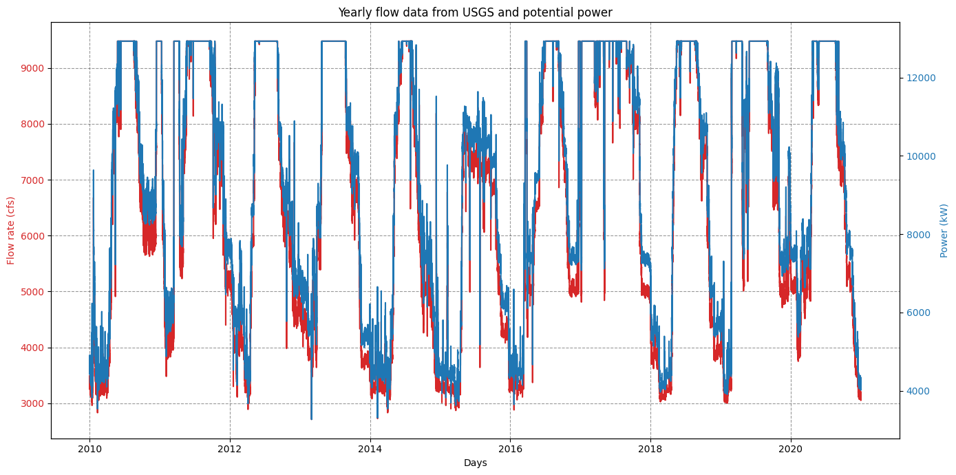
# Plot results
# Columns:  discharge_cfs   site_id     power_kW  efficiency   energy_kWh
plt.rcParams['figure.figsize'] = [14, 7]

df = hp.dataframe_output.copy()
fig, ax1 = plt.subplots()


color_plot = 'tab:red'
ax1.set_xlabel('Days')
ax1.set_ylabel('Flow rate (cfs)', color=color_plot)
ax1.plot(df['turbine_flow_cfs'], label="Flow rate", color=color_plot)
ax1.tick_params(axis='y', labelcolor=color_plot)

ax2 = ax1.twinx()  # instantiate a second axes that shares the same x-axis
color_plot2 = 'tab:blue'
ax2.set_ylabel('Power (kW)', color=color_plot2)  # we already handled the x-label with ax1
ax2.plot(df['power_kW'],label="Power", color=color_plot2)
ax2.tick_params(axis='y', labelcolor=color_plot2)
ax1.grid(True, axis='both', color='k',linestyle='--',alpha=0.4)
plt.title("Yearly flow data from USGS and potential power")
fig.tight_layout()  # otherwise the right y-label is slightly clipped
#plt.savefig(os.path.join('..','fig','usgs_twin_falls_flow_power.jpg'))
plt.show()