Querying data from the USGS National Water Information System#
The USGS National Water Information System (NWIS) provides access to surface-water data at approximately 8,500 sites. The data are served online—most in near realtime—to meet many diverse needs. For additional information regarding NWIS, visit the USGS website.
from HydroGenerate.hydropower_potential import calculate_hp_potential
import pandas as pd
import matplotlib.pyplot as plt
Use streamflow data from a USGS stream gauge.#
The USGS has a Python package (dataretrieval) designed to simplify the process of loading hydrologic data into the Python environment. dataretrieval can be pip installed into a Python environment. The example code shows how to donwload data using dataretrieval and format it for hydropower potential evaluation in HydroGenerate. The example used, and additional information, is avlaiable as a HydroShare Resource. Information about dataretrieval is avaliable directly on the USGS GitHUb Repository.
# Install dataretrieval, if it doesn't exist in Python environment, using:
# !pip install dataretrieval
# import data retrieval
from dataretrieval import nwis
# Set the parameters needed to retrieve data
siteNumber = "10109000" # LOGAN RIVER ABOVE STATE DAM, NEAR LOGAN, UT
parameterCode = "00060" # Discharge
startDate = "2010-01-01"
endDate = "2020-12-31"

# Retrieve the data
dailyStreamflow = nwis.get_dv(sites=siteNumber, parameterCd=parameterCode, start=startDate, end=endDate)
# convert to pandas dataframe
flow = pd.DataFrame(dailyStreamflow[0])
flow.head()
| site_no | 00060_Mean | 00060_Mean_cd | |
|---|---|---|---|
| datetime | |||
| 2010-01-01 00:00:00+00:00 | 10109000 | 108.0 | A |
| 2010-01-02 00:00:00+00:00 | 10109000 | 107.0 | A |
| 2010-01-03 00:00:00+00:00 | 10109000 | 106.0 | A |
| 2010-01-04 00:00:00+00:00 | 10109000 | 102.0 | A |
| 2010-01-05 00:00:00+00:00 | 10109000 | 105.0 | A |
# Use the streamflow data from a USGS stream gauge - Cont.
# The flow data for this example was created in the previous step.
head = 100 # ft
power = None
penstock_length = 120 # ft
hp_type = 'Diversion'
flow_column = '00060_Mean'  # name of the column containing the flow data

hp = calculate_hp_potential(flow= flow, rated_power= power, head= head,
                            penstock_headloss_calculation= True,
                           hydropower_type= hp_type, penstock_length= penstock_length,
                           flow_column= flow_column, annual_caclulation= True)

# Explore output
print('Design flow (cfs):', hp.design_flow)
print('Head_loss at design flow (ft):', round(hp.penstock_design_headloss, 2))
print('Turbine type:', hp.turbine_type)
print('Rated Power (Kw):', round(hp.rated_power, 2))
print('Net head (ft):', round(hp.net_head, 2))
print('Generator Efficiency:',hp.generator_efficiency)
print('Head Loss method:',hp.penstock_headloss_method)
print('Penstock length (ft):', hp.penstock_length)
print('Penstock diameter (ft):', round(hp.penstock_diameter,2))

print('\nPandas dataframe output: \n', hp.dataframe_output)
print('Annual output: \n', hp.annual_dataframe_output)
Design flow (cfs): 194.0
Head_loss at design flow (ft): 8.42
Turbine type: Crossflow
Rated Power (Kw): 1164.67
Net head (ft): 91.58
Generator Efficiency: 0.98
Head Loss method: Darcy-Weisbach
Penstock length (ft): 120.0
Penstock diameter (ft): 3.31

Pandas dataframe output:
                             site_no  00060_Mean 00060_Mean_cd    power_kW  \
datetime
2010-01-01 00:00:00+00:00  10109000       108.0             A  582.174122
2010-01-02 00:00:00+00:00  10109000       107.0             A  559.829629
2010-01-03 00:00:00+00:00  10109000       106.0             A  532.266175
2010-01-04 00:00:00+00:00  10109000       102.0             A  327.160245
2010-01-05 00:00:00+00:00  10109000       105.0             A  497.807166
...                             ...         ...           ...         ...
2020-12-27 00:00:00+00:00  10109000        91.0             A    0.000000
2020-12-28 00:00:00+00:00  10109000        85.9             A    0.000000
2020-12-29 00:00:00+00:00  10109000        83.0             A    0.000000
2020-12-30 00:00:00+00:00  10109000        82.3             A    0.000000
2020-12-31 00:00:00+00:00  10109000        90.1             A    0.000000

                           turbine_flow_cfs  efficiency    energy_kWh
datetime
2010-01-01 00:00:00+00:00             108.0    0.667042           NaN
2010-01-02 00:00:00+00:00             107.0    0.647115  13435.911095
2010-01-03 00:00:00+00:00             106.0    0.620755  12774.388208
2010-01-04 00:00:00+00:00             102.0    0.395758   7851.845891
2010-01-05 00:00:00+00:00             105.0    0.585813  11947.371983
...                                     ...         ...           ...
2020-12-27 00:00:00+00:00              91.0    0.000000      0.000000
2020-12-28 00:00:00+00:00              85.9    0.000000      0.000000
2020-12-29 00:00:00+00:00              83.0    0.000000      0.000000
2020-12-30 00:00:00+00:00              82.3    0.000000      0.000000
2020-12-31 00:00:00+00:00              90.1    0.000000      0.000000

[4018 rows x 7 columns]
Annual output:
           annual_turbinedvolume_ft3  mean_annual_effienciency  \
datetime
2010                    1306.698558                  0.439088
2011                    1794.163775                  0.713420
2012                    1428.608045                  0.579189
2013                    1080.217960                  0.229522
2014                    1275.753959                  0.440304
2015                    1198.041333                  0.302951
2016                    1359.701944                  0.505515
2017                    1876.106931                  0.776738
2018                    1402.726490                  0.582537
2019                    1441.469536                  0.585321
2020                    1319.497751                  0.458687

          total_annual_energy_KWh  revenue_M$  capacity_factor
datetime
2010                 4.509217e+06    0.262436         0.441973
2011                 8.669709e+06    0.504577         0.849765
2012                 6.167476e+06    0.358947         0.604508
2013                 2.482830e+06    0.144501         0.243356
2014                 4.546781e+06    0.264623         0.445655
2015                 3.307046e+06    0.192470         0.324141
2016                 5.282291e+06    0.307429         0.517746
2017                 9.501989e+06    0.553016         0.931341
2018                 5.965294e+06    0.347180         0.584691
2019                 6.163521e+06    0.358717         0.604120
2020                 4.704248e+06    0.273787         0.461089
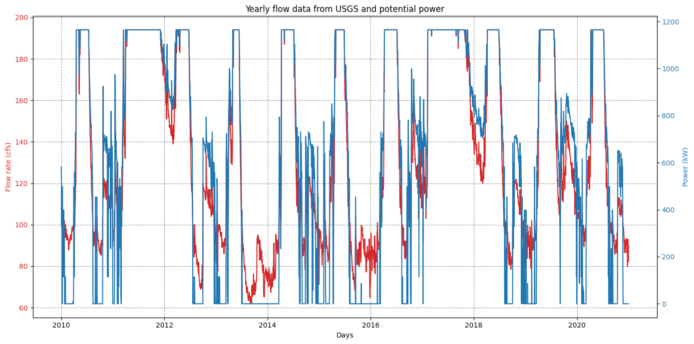
# Plot results
# Columns:  discharge_cfs   site_id     power_kW  efficiency   energy_kWh

plt.rcParams['figure.figsize'] = [14, 7]

df = hp.dataframe_output.copy()
fig, ax1 = plt.subplots()


color_plot = 'tab:red'
ax1.set_xlabel('Days')
ax1.set_ylabel('Flow rate (cfs)', color=color_plot)
ax1.plot(df['turbine_flow_cfs'], label="Flow rate", color=color_plot)
ax1.tick_params(axis='y', labelcolor=color_plot)

ax2 = ax1.twinx()  # instantiate a second axes that shares the same x-axis
color_plot2 = 'tab:blue'
ax2.set_ylabel('Power (kW)', color=color_plot2)  # we already handled the x-label with ax1
ax2.plot(df['power_kW'], label="Power", color=color_plot2)
ax2.tick_params(axis='y', labelcolor=color_plot2)
ax1.grid(True, axis='both', color='k',linestyle='--',alpha=0.4)
plt.title("Yearly flow data from USGS and potential power")
fig.tight_layout()  # otherwise the right y-label is slightly clipped
#plt.savefig(os.path.join('..','fig','usgs_twin_falls_flow_power.jpg'))
plt.show()